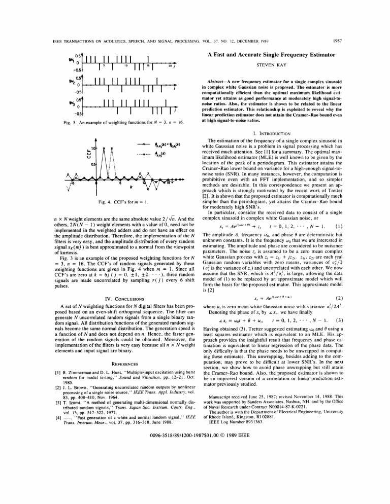
1987 IEEE TRANSACTIONS ON ACOUSTICS. SPEECH. A N D SIGNAL PROCESSING, VOL. 37. NO 12. DECEMBER 1989 A Fast and Accurate Single Frequency Estimator STEVEN KAY I l l I I IIII -0.5. I . , I I i Fig. 3. An example of weighting functions for N = 3 , n Fig. 4. CCF’s form = 16. = 1. n X N weight elements are the same absolute value 2 / & . And the others, 2 N ( N - 1) weight elements with a value of 0, need not be implemented in the weighted adders and d o not have a n effect on the amplitude distribution. Therefore, the implementation of the N filters is very easy, and the amplitude distribution of every random signal x,( mj ) is best approximated to a normal from the viewpoint of kurtosis. Fig. 3 is an example of the proposed weighting functions for N = 3, n = 16. The CCF’s of random signals generated by these weighting functions are given in Fig. 4 when m = 1. Since all three random CCF’s are zero at k = 6 j ( j = 0 , +1, f 2 , * signals are made uncorrelated by sampling r ( j ) every 6 shift pulses. - e ) , IV. CONCLUSIONS A set of N weighting functions for N digital filters has been proposed based on an even-shift orthogonal sequence. The filter can generate N uncorrelated random signals from a single binary random signal. All distribution functions of the generated random signals become the same normal distribution. The generation speed is a function of N and does not depend on n. Hence, the faster generation of the random signals could be obtained. Moreover, the implementation of the filters is very easy because all n x N weight elements and input signal are binary. REFERENCES [l] R. Zimmerman and D.L. Hunt, “Multiple-input excitation using burst random for modal testing,” Sound and Vibration, pp. 12-21, Oct. 1985. [2] J. L. Brown, “Generating uncorrelated random outputs by nonlinear processing of a single noise source,” IEEE Trans. Appl. Industry, vol. 83, pp. 408-410, NOV.1964. [3] T. Izumi, “A method of generating multi-dimensional normally distributed random signals,” Trans. Japan Soc. Instrum. Contr. Eng., vol. 13, pp. 517-522, 1977. [4] -, “Fast generation of a white and normal random signal,” IEEE Trans. Instrum. Meas., vol. 37, pp. 316-318, June 1988. Abstract-A new frequency estimator for a single complex sinusoid in complex white Gaussian noise is proposed. The estimator is more computationally efficient than the optimal maximum likelihood estimator yet attains as good performance at moderately high signal-tonoise ratios. Also, the estimator is shown to be related to the linear prediction estimator. This relationship is exploited to reveal why the linear prediction estimator does not attain the Cramer-Rao bound even at high signal-to-noise ratios. I. INTRODUCTION The estimation of the frequency of a single complex sinusoid in white Gaussian noise is a problem in signal processing which has received much attention. See [ I ] for a summary. The optimal maximum likelihood estimator (MLE) is well known to be given by the location of the peak of a periodogram. This estimator attains the Cramer-Rao lower bound on variance for a high-enough signal-tonoise ratio (SNR). In many instances, however, the computation is prohibitive even with a n F F T implementation, and so simpler methods are desirable. In this correspondence we present an approach which is strongly motivated by the recent work of Tretter [ 2 ] .It is shown that the proposed estimator is computationally much simpler than the periodogram, yet attains the Cramer-Rao bound for moderately high SNR’s. In particular, consider the received data to consist of a single complex sinusoid in complex white Gaussian noise, or X, = Ael(WOr’+@) +z, t=0,1,2;..,N-l. (1) The amplitude A, frequency WO, and phase 0 are deterministic but unknown constants. It is the frequency wo that we are interested in estimating. The amplitude and phase are considered to be nuisance parameters. The noise z, is assumed to be a zero mean complex white Gaussian process with z, = z,, + jz?,. z,,, z2, are each real Gaussian random variables with zero means, variances of u 5 / 2 ( u t is the variance of z , ) and uncorrelated with each other. W e now assume that the SNR, which is A 2 / u t , is large, allowing the data model of ( I ) to be replaced by an approximate model which will form the basis for the proposed estimator. This approximate model is [2] x, = A e J ( W @ + B + u 8 ) (2) where U, is zero mean white Gaussian noise with variance u?/2A2. Denoting the phase of x, by L X , , we have finally LX,=Wot+e+U,, t = o , 1 , 2 , - . . , ~ - 1 . (3) Having obtained (3), Tretter suggested estimating and 0 using a least squares estimator which is equivalent to an MLE. His approach provides the insightful result that frequency and phase estimation is equivalent to linear regression of the phase data. The only difficulty is that the phase needs to be unwrapped in computing these estimates. This unwrapping, besides adding to the computation, may prove to be difficult at lower SNR’s. In the next section, we show how to avoid phase unwrapping but still attain the Cramer-Rao bound. Also, the proposed estimator is shown to be an improved version of a correlation o r linear prediction estimator previously studied. Manuscript received June 25, 1987; revised November 14, 1988. This work was supported by Sanders Associates, Nashua, NH, and by the Office of Naval Research under Contract N00014-87-K-0221. The author is with the Department of Electrical Engineering, University of Rhode Island, Kingston, RI 02881. IEEE Log Number 8931363. 0096-3518/89/1200-1987$01 .OO 0 1989 IEEE 1988 IEEE TRANSACTIONS ON ACOUSTICS. SPEECH, A N D SIGNAL PROCESSING. VOL. 37. NO. 12. DECEMBER 1989 11. DERIVATION OF ESTIMATOR Assuming that we wish to estimate only the frequency, we can avoid phase unwrapping by considering the differenced phase data A, = f o r t = 0, 1, * . . ,N - LX,+I LX, (4) - 2, which becomes, from (3), AI = WO + uI+I - U,. (5) It is clear from ( 5 ) that the problem now is to estimate the mean, wo, of a colored Gaussian noise process. The process is actually a moving average with coefficients 1 and - 1. The MLE of w0. which is equivalent to the minimum variance unbiased estimator for the linear model of (9,is found by minimizing [4] J = (A N-2 Go = r=n w,A,. Note that Cy=-: w, = 1 since Bo is an unbiased estimator (at least at high SNR). The frequency estimator may further be written by using the equivalence A, = ( 10) - Lx,= Lx,*X,+I LX,+I as N-2 Go = c (11) W,LXr*X,+' r=o W ~ I ) ~ C - I (-Awol) (6) w h e r e A = [ A o A, . . . A N - 2 1 T , 1 = [ l 1 . . . I I T , a n d C i s the ( N - 1 ) X ( N - 1 ) covariance matrix of A,. The solution to this problem is well known and is - Hence, we have from (7) that with variance which follows from (8) as Var (Go) = 6 A -NN(N? - 1) U; (7) Also, it can be shown that the variance of this estimator is 1 - Var (Go) = 1TC I 1' - It remains only to explicitly evaluate Go and Var (Go). Note that Go is unbiased (let A = ool U in (7), where [ U ] , = U,+ I - U, f o r t = 0, I , 2, . . * , N - 2 ) , and that Go is a Gaussian random variable, being a linear function of the data. T o evaluate e - ' , first note that A, is a real moving average process with driving noise variance u;/2A2 and coefficients bo = I , b , = - 1. The covariance function is thus + The covariance matrix takes on the tridiagonal form ... ... .. . . . . . . . . . . . . . 2 -1 0 -1 0 0 2 -1 0 0 .*. 0 -1 , .. where min (i, j ) denotes the minimum of i and j . After some algebra, we have that 'IA2 6 4 N ( N ~- i ITc-IA = 6 4 Go = 12 N ( N ~- 1 ) c N-l t L X , r=O ~ I=O ~ WIA, N(N + 1) LX, (13) I=O which is identical to the linear regression estimator of Tretter. That (1 1) and (13) must be the same estimator is also guaranteed by the theorem that if an efficient estimator exists (i.e., it attains the Cramer-Rao bound), then it must be unique [ 7 ] . The form of the estimator given by (11) is similar to that of a previously proposed estimator as will be discussed in Section 111. It is of interest to note here that w,is a window which is symmetric about the point t = N / 2 - 1. Some examples of this window are given in Fig. I . As will be discussed shortly, it is this window which is responsible for Bo attaining the Cramer-Rao bound. If w, = 1 / N - 1 were chosen, for example, then Bo would be the samr = 0 , I , . . . , N - 2. ple mean of the measurements L X : X , + This choice would neglect the colored noise of ( 5 ) , which led to the need for C - ' in (6) and ultimately produced w, in (1 I ) . In fact, for w, = 1 / N - 1, the estimator becomes . N-2 . N-2 which although unbiased [see (3)] can be expected to exhibit a large variance due to the lack of averaging. It is easily verified that for no windowing Var (Go) = ) -~ 2 The inverse is well known with the (i, j ) element of the ( N - 1 ) X ( N - 1 ) matrix being given by [SI 1Tc-11 = N ( N 2 - But (12) is identical to the Cramer-Rao bound 161. Additionally, the least squares or MLE estimator of Tretter has also been shown to attain the Cramer-Rao bound. It is clear then that Go as given by (1 1) and Tretter's estimator must be identical. In practice, however, (1 l ) is to be preferred since it avoids phase unwrapping. T o verify this equivalence directly, we may rewrite (1 1) using (IO) as ~ - ~ 1 2 A' ( N - 1 ) -5 (14) 4. which follows by using (3). The ratio of variances is found from (12) and (14) as where N2 - 1 For large data records, this loss in performance can be substantial. 1989 IEEE TRANSACTIONS ON ACOUSTICS. SPEECH, A N D SIGNAL PROCESSING. VOL. 37. NO. 12, DECEMBER 1989 100 I 1 75 CRAMER-RA0 50 25 0 1 2 3 4 5 8 7 8 9 10 11 12 13 14 16 16 17 18 01 I I -10 10 0 20 30 Sampknunb.r. t + Nil0 40 SNR (dB) W O Fig. 2. Performancy of frequency estimators. Fig. 1 . Frequency estimator window. 111. RELATIONSHIP WITH LINEARPREDICTION ESTIMATES The frequency estimates considered in Section I1 were N-2 Go= c r=o L x:x, +I where t - (; w, = - N2 - 1 and . - 1) N 2 - used, and the mean square error versus SNR (both in decibels) determined. As a basis for comparison, the Cramer-Rao bound, which assumes an unbiased estimator, is plotted, and the performance of the MLE or location of the peak of a periodogram was also determined. The results are shown in Fig. 2 for wO/27r = 0.05. As predicted by theory for high enough SNR, the MLE as well as the weighted phase averager and weighted linear prediction estimator attain the Cramer-Rao bound. The threshold for the MLE is about -1 dB, while that for the weighted phase averager is 6 dB. The weighted linear predictor does not appear to exhibit a sharp threshold but gradually deteriorates in performance with decreasing SNR. The unweighted phase averager and linear predictor exhibit the same performance at high SNR which as predicted from (15) is about 10 loglo N / 6 = 6 dB below the Cramer-Rao bound. The threshold for the unweighted phase averager is about 6 dB, while for the linear predictor no threshold is apparent. N-2 so= ' c N - 1 r=O LX,*X,+I. It is possible to find two additional frequency estimators which are equivalent to (16) and (17) at high SNR. These are, respectively, APPENDIX OF ANGLEA N D SUMMATION OPERATORS INTERCHANGE Consider the estimators N-2 N-2 Go = L c r=O w,x:x,+I &&I)= (18) c r=o w f L x : x , + I N-2 = (42, and Go = L 1 N-2 - x:x,+I. N - 1 r=O c (19) To form these new estimators, we have interchanged the operations of taking the angle and summation. At high SNR, the performance of (18) is identical to (16), and that of (19) is identical to (17) as shown in the Appendix. It is interesting to note that (19) has been proposed by Lank, Reed, and Pollon [3] and later studied by Jackson and Tufts [8] and by Kay [9] as a linear prediction estimator. The variance of (19) is given in [3] and is identical to (14). Our results show that a windowed linear prediction estimator as given by (18) is optimal in that it achieves the Cramer-Rao bound at high SNR. At lower SNR, (16) and (18) are different estimators having distinctly different performance. The same can be said about (17) and (19). Computer simulations which will be described in Section IV show, however, that (16) provides the best overall performance. IV. COMPUTER SIMULATIONS A computer simulation was performed to compare the performance of the four estimators given in (16)-(19). We term (16) as the weighted phase averager, (17) as the unweighted phase averager, (18) as the weighted linear prediction estimator, and (19) as the linear prediction estimator. A data record of N = 24 points was fFo L wrx:xr + I where C:=i2 w , = 1. We will show that for high SNR, these two estimators are identical. At high SNR using (4) and (5) = Af = w0 LX,*X,+~ where U, = U,+ I + U, - U, so that x , * x r + , = eJw"eJ1" ;A" N-2 = c r=o N-2 W,(Wo + U,) = WO + rc= o Now consider the second estimator N-2 = WO + N-2 L C r=o w,eJr". WrU,. 1990 IEEE TRANSACTIONS ON Assuming I U , 1 << ACOUSTICS. I, N-2 ;A2’ = wo + = wo + arctan /C= 0 W , U , = WO + /C= 0 w/v/ = 46’). L C /=O W/(I + jv/) N-Z N-2 ACKNOWLEDGMENT The author would like to thank B. Musicus of the Massachusetts Institute of Technology for fruitful discussions of the work presented herein, and D. Sengupta of the University of California for performing the computer simulations. REFERENCES [I] S . Kay, Modern Spectral Estimation: Theory and Application. Englewood Cliffs, NJ: Prentice-Hall, 1988. 121 S . A. Tretter, “Estimating the frequency of a noisy sinusoid by linear regression,” IEEE Trans. Inform. Theory, vol. IT-3 1 , pp. 832-835, Nov. 1985. [3] G. W . Lank, I. S. Reed, and G. E. Pollon, “A semicoherent detection and Doppler estimation statistic,” IEEE Trans. Aerosp. Electron. Sysr., vol. AES-9, pp. 151-165, Mar. 1973. [4] S . Zacks, Paramerric Statistical Inference. New York: Pergamon, 1981. [5] M. Marcus, “Basic theorems in matrix theory,” National Bureau of Standards, Appl. Math. Series, 1960. [ 6 ] D. C. Rife and R. R. Boorstin, “Single tone parameter estimation from discrete-time observations,” IEEE Trans. Inform. Theory, vol. IT-20, pp. 591-598, Sept. 1974. 171 M. Kendall and A. Stuart, The Advanced Theory of Sratisrics I I . New York: Macmillan, 1979. [8] L. B. Jackson and D. W. Tufts, “Frequency estimation by linear prediction,” presented at ICASSP, Tulsa, OK, 1978. [9] S . Kay, “Comments on ‘Frequency estimation by linear prediction,’ * ’ IEEE Trans. Acoust., Speech, Signal Processing, vol. ASSP-21, Apr. 1979. Performance Analysis of ESPRIT and TAM in Determining the Direction of Arrival of Plane Waves in Noise BHASKAR D. RA0 AND SPEECH, A N D SIGNAL PROCESSING. VOL. 37. NO. I ? , DECEMBER 1989 Squares ESPRIT have the same mean squared error. Expressions for the asymptotic mean squared error in the estimates of the direction of arrival are derived for the methods. Simple closed-form expressions are derived for the one and two source case to get further insight. Computer simulations are provided to substantiate the analysis. I . INTRODUCTION Subspace based methods for estimating the Direction of Arrival (DOA) of plane waves in noise have been developed and studied by a number of researchers [1]-[4]. In this correspondence, wc analyze the performance of two of these methods, ESPRIT [I] and the Toeplitz Approximation Method (TAM) [3]. MUSIC was the first method that showed the benefits of using a subspace based approach [4]. Due to length and technical considerations, an evaluation of MUSIC and a comparison to the above methods is the subject of [ 5 ] . Some theoretical results comparing MUSIC and the Minimum-Norm method can be found in [6] and [7] where a characterization of the methods was done by examining the null spectrum. Our work, motivated by these papers, characterizes the error in the estimate of the direction of arrival directly. Some comparisons of MUSIC to ESPRIT can be found in [9]. ESPRIT is, like MUSIC, a general approach, and was developed to overcome some of the computation and prior information requirements of MUSIC [l], [8], [9]. Here we only consider its performance in the context of a linear equispaced sensor array. The use of TAM for DOA estimation was first suggested in [3]. A key feature of the method is that it is based on a state space model. In fact, it will be shown that for the linear equispaced sensor array case, ESPRIT can also be described using this formulation. The organization of the correspondence is as follows. First, TAM and ESPRIT are briefly reviewed and their relationship is established. It is shown that the least squares version of ESPRIT and TAM are statistically equivalent. It is then shown that, asymptotically, the estimates obtained using Least Squares ESPRIT and Total Least Squares ESPRIT have the same mean squared error. Expressions for the asymptotic mean squared error in the estimates of the DOA are then derived. The results are specialized for the one and two source case leading to interesting insights. Simulation results are presented and they support the analysis. 11. PROBLEMFORMULATION The problem of estimating the direction of arrival of M incoherent plane waves incident on a linear equispaced array of L sensors is considered in this correspondence. For the kth observation period (snapshot), the spatial samples of the signal plus noise are given by K. V. S . HARl Abstract-In this correspondence, two subspace based methods, ESPRIT and the Toeplitz Approximation Method (TAM), for estimating the direction of arrival (DOA) of plane waves in white noise in the case of a linear equispaced sensor array are evaluated. It is shown that the least squares version of ESPRIT and TAM result in the same estimate, and are statistically equivalent. It is shown that, asymptotically, the estimates obtained using Least Squares ESPRIT and Total Least Manuscript received May 17, 1988; revised February 28, 1989. This work was supported by the Army Research Office under Grant DAAL-0386-K-0107. The authors are with the AMES Department-Systems Science, University of California, San Diego, La Jolla, CA 92093. IEEE Log Number 8931337. where w, = 27r(d/X) sin Oi, d being the separation between sensors, X the wavelength of the incident signal, and 0, the direction of arrival. It is assumed that Nk is a mean zero Gaussian random vector with independent elements, i.e., E[NkNF] = atZ. The noise is assumed independent of the complex signal amplitudesplk’which are also modeled as being jointly Gaussian. The covariance matrix P of the amplitudes whose elements are P,, where Pij = E [ pik)pj*‘k’] is assumed to be of rank M and has distinct eigenvalues. In this correspondence, E [ - ] and the overbar “ - ” will be used interchangeably to denote the expectation operator. ’ ‘In this correspondence, Tis used to denote transpose, * to denote complex conjugate, H to denote complex conjugate transpose. Also ” is used to denote estimates, and the subscripts to denote parameters associated with the signal alone. 0096-3518/89/1200-1990$01.OO 0 1989 IEEE
