Multisensor-Fusion for 3D Full-Body Human Motion Capture
Gerard Pons-Moll1 , Andreas Baak2 , Thomas Helten2 , Meinard Müller2 , Hans-Peter Seidel2 , Bodo Rosenhahn1
2
1
Leibniz Universität Hannover, Germany
Saarland University & MPI Informatik, Germany
{pons,rosenhahn}@tnt.uni-hannover.de
{abaak,thelten,meinard}@mpi-inf.mpg.de
Abstract
In this work, we present an approach to fuse video with
orientation data obtained from extended inertial sensors
to improve and stabilize full-body human motion capture.
Even though video data is a strong cue for motion analysis, tracking artifacts occur frequently due to ambiguities
in the images, rapid motions, occlusions or noise. As a
complementary data source, inertial sensors allow for driftfree estimation of limb orientations even under fast motions.
However, accurate position information cannot be obtained
in continuous operation. Therefore, we propose a hybrid
tracker that combines video with a small number of inertial
units to compensate for the drawbacks of each sensor type:
on the one hand, we obtain drift-free and accurate position
information from video data and, on the other hand, we obtain accurate limb orientations and good performance under fast motions from inertial sensors. In several experiments we demonstrate the increased performance and stability of our human motion tracker.
1. Introduction
In this paper, we deal with the task of human pose tracking, also known as motion capturing (MoCap) [14]. A basic prerequisite for our system is a 3D model of the person and at least one calibrated camera view. The goal of
MoCap is to obtain the 3D pose of the person, which is
in general an ambiguous problem. Using additional a priori knowledge such as familiar pose configurations learned
from motion capture data helps considerably to handle more
difficult scenarios like partial occlusions, background clutter, or corrupted image data. There are several ways to
employ such a priori knowledge to human tracking. One
option is to learn the space of plausible human poses and
motions [2, 4, 12, 13, 21, 19]. Another option is to learn
a direct mapping from image features to the pose space
[1, 9, 19, 25]. To constrain the high dimensional space of
kinematic models, a major theme of recent research on human tracking has been dealing with dimensionality reduction [27, 28]. Here, the idea is that a typical motion pat-
978-1-4244-6985-7/10/$26.00 ©2010 IEEE
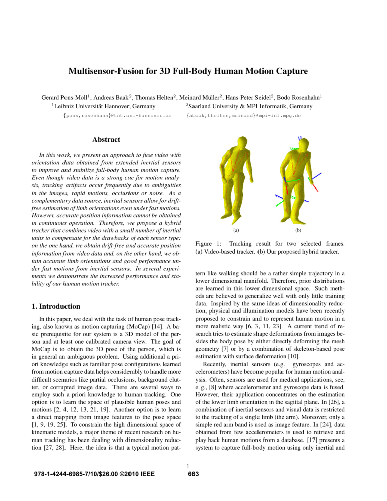
(a)
(b)
Figure 1: Tracking result for two selected frames.
(a) Video-based tracker. (b) Our proposed hybrid tracker.
tern like walking should be a rather simple trajectory in a
lower dimensional manifold. Therefore, prior distributions
are learned in this lower dimensional space. Such methods are believed to generalize well with only little training
data. Inspired by the same ideas of dimensionality reduction, physical and illumination models have been recently
proposed to constrain and to represent human motion in a
more realistic way [6, 3, 11, 23]. A current trend of research tries to estimate shape deformations from images besides the body pose by either directly deforming the mesh
geometry [7] or by a combination of skeleton-based pose
estimation with surface deformation [10].
Recently, inertial sensors (e.g. gyroscopes and accelerometers) have become popular for human motion analysis. Often, sensors are used for medical applications, see,
e. g., [8] where accelerometer and gyroscope data is fused.
However, their application concentrates on the estimation
of the lower limb orientation in the sagittal plane. In [26], a
combination of inertial sensors and visual data is restricted
to the tracking of a single limb (the arm). Moreover, only a
simple red arm band is used as image feature. In [24], data
obtained from few accelerometers is used to retrieve and
play back human motions from a database. [17] presents a
system to capture full-body motion using only inertial and
1
663
magnetic sensors. While the system in [17] is very appealing because it does not require cameras for tracking, the
subject has to wear a suit with at least 17 inertial sensors,
which might hamper the movement of the subject. In addition, long preparation time before recording is needed.
Moreover, inertial sensors suffer from severe drift problems
and cannot provide accurate position information in continuous operation.
where exp(θ
ω ) is the exponential map from so(3) to SO(3)
which can be calculated using the Rodriguez formula
1.1. Contributions
The dynamics of the subject are modeled by a kinematic
chain F , which describes the motion constraints of an articulated rigid body such as the human skeleton [5]. The underlying idea behind a kinematic chain is that the motion of
a body segment is given by the motion of the previous body
segment in the chain and an angular rotation around a joint
axis. Specifically, the kinematic chain is defined with a 6
DoF (degree of freedom) root joint representing the global
rigid body motion and a set of 1 DoF revolute joints describing the angular motion of the limbs. Joints with higher
degrees of freedom like hips or shoulders are represented by
concatenating two or three 1 DoF revolute joints. The root
joint is expressed as a twist of the form θξ with the rotation axis orientation, location, and angle as free parameters.
Revolute joints are expressed as special twists with no pitch
of the from θj ξj with known ξj (the location and orientation of the rotation axis as part of the model representation).
Therefore, the full configuration of the kinematic chain is
completely defined by a (6 + n) vector of free parameters
Even using learned priors from MoCap data, obtaining
limb orientations from video is a difficult problem. Intuitively, because of the cylindrical shape of human limbs, different limb orientations project to very similar silhouettes in
the images. These orientation ambiguities can be easily captured by the inertial sensors but accurate positions cannot
be obtained. Therefore, we propose to use a small number
of sensors (we use only five) fixed at the body extremities
(neck, wrists and ankles) as a complementary data source
to visual information. One the one hand, we obtain stable
and drift-free accurate position information from video data
and, on the other hand, we obtain accurate limb orientations
from the inertial sensors. In this work, we present how to
integrate orientation data from sensors in a contour-based
video motion capture algorithm. In several experiments, we
show the improved performance of tracking with additional
small number of sensors.
exp(θb
ω) = I + ω
b sin(θ) + ω
b 2 (1 − cos(θ)).
Note that only sine and cosine functions of real numbers
need to be computed.
2.2. Kinematic Chains
2. Twists and Exponential Maps
Θ := (θξ, θ1 , . . . , θn )
This section recalls the basics of twists and exponential
maps, for further details see [16]. Every 3D rigid motion
can be represented by a homogeneous matrix M ∈ SE(3).
„
M=
«
r
,
1
R
01×3
(1)
where R ∈ SO(3) is a rotation matrix and r ∈ R3 is
a translation. For each matrix M ∈ SE(3) there is a
corresponding twist in the tangent space se(3). An element of se(3) can either be represented by θξ, θ ∈ R and
ξ ∈ R6 = {(v, ω)|v ∈ R3 , ω ∈ R3 , ω2 = 1} or by
θξb = θ
„
ω
b
01×3
v
0
«
∈ R4×4 ,
(2)
where ω
is the skew-matrix representation of ω. In the form
ξ and ξ are referred to as normalized twists, and θ
θξ or θξ,
expresses the velocity of the twist.
2.1. From Twist to Homogeneous Matrix
Elements from se(3) are mapped to SE(3) using the exponential map for twists
b =
M = exp(θξ)
„
exp(θb
ω)
01×3
(I − exp(θb
ω ))(b
ω v + ωω T vθ)
1
«
(3)
(4)
(5)
as described in [18]. Now, for a given point x ∈ R3 on the
kinematic chain, we define J (x) ⊆ {1, . . . , n} to be the
ordered set that encodes the joint transformations influencing x. Let X = ( x1 ) be the homogeneous coordinate of x
and denote π as the associated projection with π(X) = x.
Then, the transformation of a point x using the kinematic
chain F and a parameter vector Θ is defined by
ˆ
FΘ (x) = π(g(Θ)X) = π(exp(θξ)
Y
exp(θj ξˆj )X). (6)
j∈J (x)
Here, FΘ : R3 → R3 is the function representing the
total rigid body motion g(Θ) of a certain segment in the
chain. Equation (6) is commonly known as the product of
exponentials formula [16], denoted throughout this paper
as FΘ . In our tracking system, we always seek for differential twist parameters represented in global frame coordinates Θd , subsequently we accumulate the motion to obtain
the new absolute configuration in body coordinates Θ(t).
Therefore, we have our current configuration at time t − 1
given by Θ(t − 1) and seek for the update Θd to find Θ(t).
Recall that Θ(t) is the vector of twist parameters that represent the map between the body and the global frame at
time t. However, at each iteration we update the model and
664
Θ(t)
XB
XB
Θ(t − 1)
Θd
...
XT (t − 1)
XT (t)
(a)
Frame 0
Frame t-1
Figure 2: Absolute twists in continuous line and differential
twists in dashed line. X T denotes a point in global coordinates and X B denotes a point in body coordinates.
the corresponding twists with the current Θ(t − 1) obtaining the current configuration in global coordinates. Then,
we seek for the transformation g T (Θd ) that will transform
the model configuration at frame t − 1 in global coordinates
to the model configuration at frame t also in global coordinates. For example, given a point in global coordinates
X T (t − 1), we would obtain the point in the next time t as
g T (Θd )X T (t − 1) = X T (t)
(b)
(c)
Frame t
(7)
where Θd are the differential twist parameters at time t in
the global frame, see Figure 2. Intuitively, we can think
of g T (Θd ) not as a change of coordinates but rather as the
twist parameters that give us the instantaneous angular and
linear velocity at time t for a point in the global frame. For
simplicity, let us denote the differential twist parameters in
global coordinates by Θ.
3. Video-based Tracker
In order to relate the surface model to the human’s images we find correspondences between the 3D surface vertices and the 2D image contours obtained with background
subtraction, see Figure 3. We first collect 2D-2D correspondences by matching the projected surface silhouette with the
background subtracted image contour. Thereby, we obtain
a collection of 2D-3D correspondences since we know the
3D counterparts of the projected 2D points of the silhouette.
In the presented experiments we only use the silhouettes as
image features. We then minimize the distance between the
transformed 3D points FΘ (Xi ) and the projection rays defined by the 2D points pi . This gives us a point-to-line constraint for each correspondence. Defining Li = (ni , mi ) as
the 3D Plücker line with unit direction ni and moment mi
of the corresponding 2D point pi , the point to line distance
Figure 3: (a) Original Image, (b) Background subtracted
image, (c) Projected surface mesh after convergence.
di can be expressed as
di = FΘ (Xi ) × ni − mi (8)
Similar to Bregler et al. [5] we now linearize the Equation
bk
= ∞ (θξ)
by using exp(θξ)
k=0 k! . With I as identity matrix,
this results in
π((I +
X
θj ξbj ) Xi ) × ni − mi = 0 .
(9)
j∈J (x)
Having N correspondences, we minimize the sum of
squared point-to-line distances di
arg min
Θ
N
X
di 2 = arg min
i=1
Θ
N
X
FΘ (Xi ) × ni − mi 2 (10)
i=1
which after linearization can be re-ordered into an equation
of the form A1 Θ = b1 , see Figure 4. Collecting a set of
such equations leads to an over-determined system of equations, which can be solved using numerical methods like the
Householder algorithm. The Rodriguez formula can be applied to reconstruct the group action g from the estimated
twists θj ξj . Then, the 3D points can be transformed and the
process is iterated until convergence. The used video-based
tracker is similar to the one presented in [18].
4. Hybrid Tracker
The input of our tracking system consists of:
• Rigid surface mesh of the actor obtained from a laser
scanner
• Multi-view images obtained by a set of calibrated and
synchronized cameras
• Global orientation data coming from the sensors
We used five inertial sensors fixed at the body extremities
(wrists, lower legs, and neck). The final goal is to manipulate the available data in order to relate it linearly (see Figure 4) to the differential kinematic chain parameters Θ that
determine the motion from two consecutive frames.
665
Sensor Orientation
3D-3D Vector Corr.
A1 Θ = b1
AΘ = b
Image Silhouettes
2D-3D Point Corr.
A2 Θ = b2
Figure 4: Linear equations derived from orientation data
and image silhouettes are combined into a linear equation
system.
Figure 5: Global frames: tracking frame F T and inertial
frame F I . Local frame: sensor frame F S .
5. Integration of Sensor Data
5.1. Sensor Data
In our experiments, we use an orientation estimation device MTx provided by XSens [29]. An Xsens MTx unit
provides two different streams of data: three dimensional
local linear acceleration aS and local rate of turn or angular velocity ω S . Orientation data can be obtained from the
angular velocity ω(k) provided by the sensor units. Besides
angular velocity, the MTx units provide a proprietary algorithm that can accurately calculate absolute orientations
relative to a static global frame F I , which we will refer to
as inertial frame. The inertial frame F I is computed internally in each of the sensor units in an initial static position
and is defined as follows: The Z axis is the negative direction of gravity measured by the internal accelerometer. The
X axis is the direction of the magnetic north pole measured
by a magnetometer. Finaly, the Y axis is defined by the
cross product Z × X. For each sensor, the absolute orientation data is provided by a stream of quaternions that define, at every frame, the map or coordinate transformation
from the local sensor coordinate system to the global one
q IS (t) : F S ⇒ F I . Unfortunately, the world frame defined
in our tracking system differs from the global inertial frame.
The tracking coordinate frame F T is defined by a calibration cube placed in the recording volume, in contrast to the
inertial coordinate frame which is defined by the gravity and
magnetic north directions. Therefore, in order to be able to
integrate the orientation data from the inertial sensors into
our tracking system, we must know the rotational offset q T I
between both worlds, see Figure 5.
Since the Y axis of the cube is perpendicular to the
ground and so is gravity, the Y axis of the tracking frame
and the Z axis of the inertial frame are aligned. Therefore,
q T I is a one parametric planar rotation that can be estimated
beforehand using a calibration sequence. Thus, we can easily transform the quaternions so that they define a map from
the local sensor frame to the tracking frame F T :
q T S = q T I ◦ q IS
where ◦ denotes quaternion multiplication [20].
(11)
5.2. Integration of Orientation Data into the Videobased Tracker
In this section we explain how to integrate the orientation data from the sensors as additional equations that
can be appended into the big linear system, see Figure 4.
Here we have to be very careful and know, at all times, in
which frame the rotation matrices are defined. Three coordinate systems are involved: the global tracking frame
F T , the body frame F B (the local frame of a segment in
the chain, e.g. the leg), and the sensor frame F S . Recall from Sect. 5.1 that the orientation data is given as a
quaternion q T S (t) : F S → F T defining the transformation
from the local sensor frame F S to the global tracking frame
F T , which we will refer to as ground-truth orientation. In
order to relate the orientation data to the differential twist
parameters Θ, we will compare the ground-truth orientations q T S (t) of each of the sensors with the estimated sensor
orientations from the tracking procedure q̂ T S (t), which we
will denote as tracking orientation. For the sake of simplicity in the operations, we consider from now on the groundtruth orientation q T S to be represented as a rotation matrix
3 × 3 (quaternions can be easily transformed to rotation matrices [20]). The columns of the rotation matrix q T S are
simply the sensor basis axes in world coordinates. Let us
also define R(Θ(t)) as the total accumulated motion of a
body segment at time t, i.e. R(Θ(t)) : F B → F T . For the
sake of clarity we will drop the dependency of Θ and just
write R(t). The transformation from the sensor frame to the
body frame q D (t) : F S → F B is constant during tracking
because the sensor and body frame are rigidly attached to
the body segment and move together. Thus, we can compute this rotational displacement q D in the first frame by
q D = R(0)−1 q T S (0) ,
(12)
where R(0) is the accumulated motion of the body part in
the first frame. Now consider the local rotation RB (Θ) of
frame F B from time t − 1 to time t, see Figure 6. The
rotation RB (Θ) defined in the body frame is related to the
rotation RT (Θ) defined in the global frame by the adjoint
666
transformation AdR−1 (t−1)
RB (Θ) = R(t − 1)−1 RT (Θ)R(t − 1)
Thereby, the tracking orientation q̂
D
S q
RB
FtB =⇒
TS
B R(t−1)
Ft−1
=⇒
R(t ¡ 1)
(13)
RB (£)
FB
FB
FB
is given by the longer
F , see Figure 6. Now
path F =⇒
we can compare this transformation matrix to the groundtruth orientation given by the sensors q T S
T
R(t − 1)RB (Θ)q D = q T S (t) .
FT
R(0)
qD
(14)
qT S (0)
Substituting RB (Θ) by its expression in (13) it simplifies to
RT (Θ)R(t − 1)q D = q T S (t) .
t¡1
0
FS
0
(15)
t
qD
qD
FS
FS
t¡1
t
qT S (t)
Therefore, for each sensor s, we can minimize the norm of
both matrices with respect to Θ
arg min
Θ
5 ‚
‚
X
‚
‚ T
D
TS
‚Rs (Θ)Rs (t − 1)qs − qs (t)‚ .
(16)
s=1
Equation (16) can again be reordered into the form of
A2 Θ = b2 and integrated into the linear system as soft constrains, see Figure 4. Nonetheless, it is interesting to take a
closer look at equation (15). Substituting the rotational displacement q D in equation (15) by its expression in equation
(12) we obtain
RT (Θ)R(t − 1)R(0)−1 q T S (0) = q T S (t) .
Figure 6: Integration of orientation data into the videobased tracker. Ground-truth orientation: clockwise down
path from F S at time t to F T . Tracking orientation: anticlockwise upper path from F S at time t to F T .
twist formulation. Being x̂(t−1), ŷ(t−1), ẑ(t−1) the tracking orientation basis axes in frame t−1, and x(t), y(t), z(t)
ground-truth orientation basis axes in the current frame t,
the constraint equations are
2
(17)
R (Θ)4x̂(t − 1)
Expressing R(t − 1) in terms of instantaneous rotations
RT (Θ)(
0
Y
RT (j))R(0)−1 q T S (0) = q T S (t) .
Simplifying R(0)−1 we obtain
1
Y
RT (j))q T S (0) = q T S (t) .
(19)
j=t−1
the columns of the matrix (
ẑ(t − 1)5=4x(t)
y(t)
z(t)5
which can be linearized similarly as we did in the videobased tracker with image points to mesh points correspondences (2D-point to 3D-point). The difference now is that
since we rotate vectors, only the rotational component of the
twists is needed. For example, the equation for the X-axis
correspondence (x̂(t − 1), x(t)) would be
RT (j))q T S (0) are simply the
j=t−1
coordinates of the sensor axis in the first frame (columns of
q T S (0)), rotated by the accumulated tracking motion from
the first frame forward (i.e. not including the initialization
motion in frame 0). This last result was very much expected and the interpretation is the following: if we have
our rotation matrices defined in a reference frame F T , we
can just take the sensor axes in global coordinates in the
first frame (columns of q T S (0)) and rotate them at every
frame by the instantaneous rotational motions of the tracking. This will result in the estimated sensor axes in world
coordinates, which is exactly the tracking orientation defined earlier in this Section. Therefore, the problem can be
simplified to additional 3D-vector to 3D-vector constraint
equations which can be very conveniently integrated in our
X
(I +
This last equation has a very nice interpretation because
1
Y
ŷ(t − 1)
3
(20)
(18)
j=t−1
RT (Θ)(
3 2
T
θj ω
cj )x̂(t − 1) = x(t)
(21)
j∈J (x)
which depends only on θj ω
j . In other words, the constraint
equations do not depend at all on the joint axis location nor
in the translational motion of the body. This implies that
we can integrate the sensor information into the tracking
system independently of the initial sensor orientation and
location at the body limb.
6. Experiments
In this section, we evaluate our multisensor-fusion approach for motion tracking by comparing the video-based
tracker with our proposed hybrid tracker. Learning-based
stabilization methods or joint angle limits can also be integrated into the video-based tracker. However, we did
not include further constraints into the video-based tracker
667
dquat [deg]
150
100
50
50
100
150
200
250
300
350
400
450
Frames
Figure 7: Error curves for video-based tracking (red) and
hybrid tracking (black), referring to the orientations of the
left lower leg for a hopping and jumping motion sequence.
to demonstrate a general weakness of silhouette-based approaches. We note that the video-based tracker works well
for many sequences, however in these experiments we focus on the occasions where it fails. Even though benchmarks for video-based tracking are publicly available [22],
so far no data set comprising video as well as inertial data
exist for free use. Therefore, for our experiments, we generated a data set consisting of 54 takes each having a length
of roughly 15 seconds. In total, more than 10 minutes of
tracking results were used for our validation study, which
amounts to more than 24 thousand frames at a frame rate
of 40 Hz. All takes have been recorded in a lab environment using eight calibrated video cameras and five inertial
sensors fixed at the two lower legs, the two hands, and the
neck. Our evaluation data set comprises various actions including standard motions such as walking, sitting down and
standing up as well as fast and complex motions such as
jumping, throwing, arm rotations, and cartwheels. For each
of the involved four actors, we also generated a 3D mesh
model using a laser scanner.
For a given tracking procedure, we introduce a framewise error measure by considering the angular distance between the two orientations q T S and q̂ T S , see Sect. 5.2. This
angular distance measured in degrees is defined by the formula
dquat (q T S , q̂ T S ) =
˛D
E˛
360
˛
˛
arccos ˛ q T S , q̂ T S ˛ .
π
(22)
For a given motion sequence, we compute the error measure
for each frame yielding an error curve.
In Figure 7, such error curves are shown for two different
tracking procedures using the original video-based tracker
(red) and the enhanced hybrid tracker (black). For the
video-based tracking, there are large deviations between the
ground-truth orientations and tracking orientations roughly
starting with frame 200. Actually, as a manual inspection
revealed, the actor performs in this moment a sudden turn
resulting in a failure of the video-based tracking, where the
left leg was erroneously twisted by almost 180 degrees. In
contrast, the hybrid tracker could successfully track the entire sequence. This is also illustrated by Figure 8. Similarly, the figure also shows a tracking error in the right
(a)
(b)
Figure 8: Tracking result for video-based tracking (a) and
hybrid tracking (b) for frame 450 of the motion sequence
used in Figure 7. Ground-truth orientations in solid lines
and tracking orientations in by dashed lines.
hand, which is corrected by the hybrid tracker as well. As
a second example, we consider a very fast motion, where
an actor first rotates his right and afterwards his left arm.
Figure 9 shows the error curves for left and right hand for
each of the tracking procedures. The curves reveal that the
video-based tracker produced significant orientation errors
in both hands. This shows that the hand orientations cannot
be captured well considering only visual cues. Again, the
hybrid tracker considerably improved the tracking results,
see also Figure 10. These examples demonstrate how the
additional orientation priors resolve ambiguities from image cues. To estimate the quality of our hybrid tracker on
more sequences, we computed the error measures (for lower
legs, the two hands, and the neck) for each of the five sensors for all sequences and each actor of the data set. A total
of 120210 error measures were computed separately for the
hybrid and video tracker. We denote mean values and standard deviations of our error measure by μV , σV and μH ,
σH for the video-based and hybrid tracker, respectively. As
summarized in Table 1, the sequences of each actor have
been improved significantly, dropping the mean error from
30◦ to 13◦ . This is also supported by the standard deviations. Let τ (s) denote the percentage of frames where at
least one of the five sensors shows an error of more than s
degrees. To show the percentage of corrected severe tracking errors, we computed τV (45) and τH (45) for every actor,
see Tab. 1. As it turns out, most of the tracking errors are
corrected, dropping the percentage of erroneously tracked
frames from 19.29% to 2.51% of all frames. These findings
are supported by the normalized histograms of the occurring values of the error measure, see Fig. 11. Furthermore,
the hybrid tracker does not increase the computation time
668
dquat [deg]
150
100
50
100
200
300
400
500
600
700
800
(a)
(b)
0.06
0.06
0.04
0.04
0.02
0.02
0
900
0
50
100
150
0
(d)
150
0.06
0.06
100
0.04
0.04
50
0.02
0.02
dquat [deg]
(c)
0
100
200
300
400
500
600
700
800
900
0
50
(a)
(b)
(c)
(d)
Figure 10: Tracking result and orientations for two selected
frames of the sequence used in Figure 9. (a),(c) Video-based
tracking. (b),(d) Hybrid tracking.
of the video-based tracker which is less than 4 s per frame.
One reason for the large amount of corrected errors is
that the orientation of limbs is hard to estimate from silhouettes, since the cylindrical shape projects to the same silhouettes in many orientations. By combining the visual with
orientation cues, these ambiguities are resolved, resulting
in a largely improved performance with the hybrid tracker.
7. Conclusions
In this paper, we presented an approach for stabilizing
full-body markerless human motion capturing using a small
number of additional inertial sensors. Generally, the goal
of reconstructing a 3D pose from 2D video data suffers
from inherent ambiguities. We showed that a hybrid approach combining information of multiple sensor types can
resolve such ambiguities, significantly improving the tracking quality. In particular, our orientation-based approach
could correct tracking errors arising from rotationally symmetric limbs. Using only a small number of inertial sensors
fixed at outer extremities stabilized the tracking for the entire underlying kinematic chain.
In the future, we plan to extend our tracker to also make
use of acceleration data and rate of turn data, which seem
150
0
0
dquat [deg]
Frames
Figure 9: Error curves for video-based tracking (red) and
hybrid tracking (black) obtained for an arm rotation sequence (first performed by the right and then by the left
arm). Top: Left hand. Bottom: Right hand.
100
0
50
100
150
50
100
150
dquat [deg]
Figure 11: Normalized histogram, for each actor, of quaternion distances comparison for the whole database.
[deg]
[deg]
[deg]
[deg]
Actor 1
26.10
11.50
33.79
9.89
Actor 2
40.80
14.86
46.99
13.01
Actor 3
26.20
13.98
29.23
12.25
Actor 4
31.10
13.85
38.07
14.43
Average
30.29
13.47
37.08
12.28
τV (45) [%]
τH (45) [%]
14.27
0.47
29.50
3.33
16.53
2.12
19.42
6.45
19.29
2.51
μV
μH
σV
σH
Table 1: Mean values μ and standard deviations σ for videobased (V ) and hybrid (H) tracker for all sequences of the
database, separated by actor. Percentage of large tracking
errors denoted by τ (45).
to be ideally suited to stabilize tracking in outdoor settings,
for fast motions, and in the presence of occlusions. To this
end, we need suitable strategies that do not destabilize the
tracking process in the presence of sensor noise and local
artifacts. Furthermore, we want to investigate in how far
such fusion techniques make monocular tracking feasible.
Finally, we make the multimodal data set used in this paper publicly available at [15] to further support this line of
research.
Acknowledgments. This work has been supported by the German
Research Foundation (DFG CL 64/5-1 and DFG MU 2686/3-1).
Meinard Müller is funded by the Cluster of Excellence on Multimodal Computing and Interaction.
References
[1] A. Agarwal and B. Triggs. Recovering 3D human pose from
monocular images. IEEE TPAMI, 28(1):44–58, 2006.
[2] A. Baak, B. Rosenhahn, M. Müller, and H.-P. Seidel. Stabilizing motion tracking using retrieved motion priors. In IEEE
ICCV, pages 1428–1435, sep 2009.
[3] A. Balan, M. Black, H. Haussecker, and L. Sigal. Shining a
light on human pose: On shadows, shading and the estimation of pose and shape. In IEEE ICCV, volume 1, 2007.
[4] A. Balan, L. Sigal, M. Black, J. Davis, and H. Haussecker.
Detailed human shape and pose from images. In IEEE
CVPR, pages 1–8, 2007.
669
Figure 12: Examples of tracking results with our proposed hybrid tracker
[5] C. Bregler, J. Malik, and K. Pullen. Twist based acquisition and tracking of animal and human kinematics. IJCV,
56(3):179–194, 2004.
[6] D. Brubaker M. A., Fleet and A. Hertzmann. Physics-based
person tracking using the Anthropomorphic Walker. In IJCV
(in press), 2010.
[7] E. de Aguiar, C. Stoll, C. Theobalt, N. Ahmed, H. Seidel,
and S. Thrun. Performance capture from sparse multi-view
video. ACM Transactions on Graphics, 27(3):98, 2008.
[8] H. Dejnabadi, B. Jolles, E. Casanova, P. Fua, and
K. Aminian. Estimation and visualization of sagittal kinematics of lower limbs orientation using body-fixed sensors.
IEEE TBME, 53(7):1382–1393, 2006.
[9] A. Elgammal and C. Lee. Inferring 3D body pose from silhouettes using activity manifold learning. In IEEE CVPR,
volume 2, 2004.
[10] J. Gall, C. Stoll, E. de Aguiar, C. Theobalt, B. Rosenhahn,
and H. Seidel. Motion capture using joint skeleton tracking
and surface estimation. IEEE CVPR, 2009.
[11] P. Guan, A. Weiss, A. Balan, and M. Black. Estimating Human Shape and Pose from a Single Image. In IEEE ICCV,
volume 1, 2009.
[12] L. Herda, R. Urtasun, and P. Fua. Implicit surface joint limits
to constrain video-based motion capture. In LNCS, volume
3022, pages 405–418, 2004.
[13] S. Ioffe and D. Forsyth. Human tracking with mixtures of
trees. In IEEE ICCV, volume 1, pages 690–695, 2001.
[14] T. Moeslund and E. Granum. A survey of computer vision
based human motion capture. CVIU, 81(3), 2001.
[15] Multimodal
Human
Motion
Database
MPI08.
http://www.tnt.uni-hannover.de/project/MPI08 Database/.
[16] R. Murray, Z. Li, and S. Sastry. Mathematical Introduction
to Robotic Manipulation. CRC Press, Baton Rouge, 1994.
[17] D. Roetenberg, H. Luinge, and P. Slycke. Xsens MVN:
Full 6DOF Human Motion Tracking Using Miniature Inertial Sensors.
[18] B. Rosenhahn, T. Brox, and H. Seidel. Scaled motion dynamics for markerless motion capture. In IEEE CVPR, pages
1–8, 2007.
[19] G. Shakhnarovich, P. Viola, and T. Darrell. Fast pose estimation with parameter-sensitive hashing. In IEEE ICCV, page
750, 2003.
[20] K. Shoemake. Animating rotation with quaternion curves.
ACM SIGGRAPH, 19(3):245–254, 1985.
[21] H. Sidenbladh and M. Black. Learning the statistics of people in images and video. IJCV, 54(1):183–209, 2003.
[22] L. Sigal and M. Black.
HumanEva: Synchronized
video and motion capture dataset for evaluation of articulated human motion.
Technical Report CS-0608, Brown University, USA, 2006.
Available at
http://vision.cs.brown.edu/humaneva/ .
[23] L. Sigal, M. Vondrak, and O. Jenkins. Physical Simulation
for Probabilistic Motion Tracking. In IEEE CVPR, 2008.
[24] R. Slyper and J. Hodgins. Action capture with accelerometers. In ACM SIGGRAPH/Eurographics, SCA, 2008.
[25] C. Sminchisescu, A. Kanaujia, Z. Li, and D. Metaxas. Discriminative density propagation for 3d human motion estimation. In IEEE CVPR, volume 1, page 390, 2005.
[26] Y. Tao, H. Hu, and H. Zhou. Integration of vision and inertial
sensors for 3d arm motion tracking in home-based rehabilitation. IJRR, 26(6):607, 2007.
[27] R. Urtasun, D. Fleet, and P. Fua. 3D people tracking with
Gaussian process dynamical models. In IEEE CVPR, pages
238–245, 2006.
[28] J. Wang, D. Fleet, and A. Hertzmann. Gaussian process dynamical models for human motion. IEEE TPAMI, 30(2):283–
298, 2008.
[29] Xsens Motion Technologies. http://www.xsens.com/, Accessed November 19th, 2009.
670
