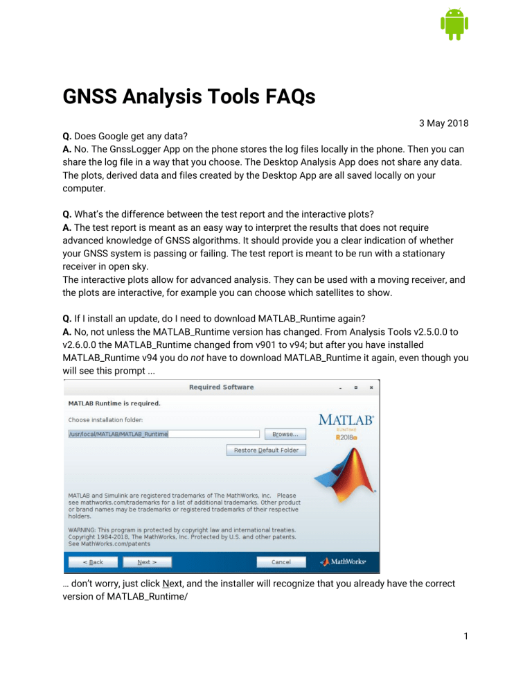
GNSS.Analysis.Tools инструкция

GNSS Analysis Tools FAQs
3 May 2018
Q.​ Does Google get any data?
A.​ No. The GnssLogger App on the phone stores the log files locally in the phone. Then you can
share the log file in a way that you choose. The Desktop Analysis App does not share any data.
The plots, derived data and files created by the Desktop App are all saved locally on your
computer.
Q.​ What’s the difference between the test report and the interactive plots?
A.​ The test report is meant as an easy way to interpret the results that does not require
advanced knowledge of GNSS algorithms. It should provide you a clear indication of whether
your GNSS system is passing or failing. The test report is meant to be run with a stationary
receiver in open sky.
The interactive plots allow for advanced analysis. They can be used with a moving receiver, and
the plots are interactive, for example you can choose which satellites to show.
Q.​ If I install an update, do I need to download MATLAB_Runtime again?
A.​ No, not unless the MATLAB_Runtime version has changed. From Analysis Tools v2.5.0.0 to
v2.6.0.0 the MATLAB_Runtime changed from v901 to v94; but after you have installed
MATLAB_Runtime v94 you do n
​ ot​ have to download MATLAB_Runtime it again, even though you
will see this prompt ...
… don’t worry, just click N
​ ​ext, and the installer will recognize that you already have the correct
version of MATLAB_Runtime/
1
Q.​ How is pseudorange smoothing done in the Gnss Analysis Tool?
A​. For details of the mathematics of pseudorange smoothing within the GNSS Analysis Tool,
read the section "Raw Measurements and Derived Data" of the attached “Inside GNSS” article.
This gives details of how we do the smoothing​:
http://insidegnss.com/gnss-analysis-tools-from-google/
To get the results of smoothing from the tool, click on [Write Data to File] in the Gnss Analysis
Tool GUI and you will get the smoothed pseudoranges for your log file.
Q​. What’s the difference between "GNSS receiver clock rate” (in the Analysis Report), “Frequency
drift” (Interactive plot), and “DriftNanosPerSecond” (in the gnss_log*.txt and raw.csv files)?
A​. They are different estimates of the same thing:
DriftNanosPerSecond is the real-time estimate of the receiver clock frequency offset (or drift),
as reported by the receiver in the Raw Measurement API.
“Frequency drift” in the Interactive Plots is the Analysis Tool estimate of the same value,
computed using the Reference Pvt:
“|GNSS receiver clock rate|, max” in the reports, is the maximum absolute value of the above
plot:
2
Q​. How do you calculate GNSS receiver clock bias and GNSS receiver clock frequency drift?
A​. Receiver clock bias is shown by the Analysis Tool in a plot like this:
The values are worked out at each epoch as follows:
For each satellite, the receiver clock bias is estimated as the measured pseudorange minus the
expected pseudorange (calculated using the Reference PVT shown in the GUI). The values for
several high elevation satellites are averaged. The satellites that are used are printed in the
above plot ​“Clock bias computed usings SVs: …”
3
GNSS receiver clock frequency drift is computed in a similar way. At each epoch that the clock
is continuous: for each satellite, the receiver clock frequency is estimated as the measured
pseudorange-rate minus the expected pseudorange-rate (calculated using the reference
velocity: either zero, if the receiver is stationary, or read from the NMEA file provided). The
values for several high elevation satellites are averaged. The satellites that are used are printed
in the Frequency drift plot.
After estimating receiver clock bias and frequency at each epoch, these values are filtered to
produce the final result shown in the plots.
The results of these calculations are available when you click [Write Data to File], the clock bias
and frequency values appear in the g
​ nss_log*.derived​ file, in the rows labeled “CLOCK”.
4